Introduction
Welcome to the Cyclistic bike-share analysis case study! In this case study, you will perform many real-world tasks of a junior data analyst. You will work for a fictional company, Cyclistic, and meet different characters and team members. In order to answer the key business questions, you will follow the steps of the data analysis process: ask, prepare, process, analyze, share, and act. Along the way, the Case Study Roadmap tables — including guiding questions and key tasks — will help you stay on the right path. By the end of this lesson, you will have a portfolio-ready case study. Download the packet and reference the details of this case study anytime. Then, when you begin your job hunt, your case study will be a tangible way to demonstrate your knowledge and skills to potential employers.
Scenario
You are a junior data analyst working in the marketing analyst team at Cyclistic, a bike-share company in Chicago. The director of marketing believes the company’s future success depends on maximizing the number of annual memberships. Therefore, your team wants to understand how casual riders and annual members use Cyclistic bikes differently. From these insights, your team will design a new marketing strategy to convert casual riders into annual members. But first, Cyclistic executives must approve your recommendations, so they must be backed up with compelling data insights and professional data visualizations.
Characters and teams
● Cyclistic: A bike-share program that features more than 5,800 bicycles and 600 docking stations. Cyclistic sets itself apart by also offering reclining bikes, hand tricycles, and cargo bikes, making bike-share more inclusive to people with disabilities and riders who can’t use a standard two-wheeled bike. The majority of riders opt for traditional bikes; about 8% of riders use the assistive options. Cyclistic users are more likely to ride for leisure, but about 30% use them to commute to work each day.
● Lily Moreno: The director of marketing and your manager. Moreno is responsible for the development of campaigns and initiatives to promote the bike-share program. These may include email, social media, and other channels.
● Cyclistic marketing analytics team: A team of data analysts who are responsible for collecting, analyzing, and reporting data that helps guide Cyclistic marketing strategy. You joined this team six months ago and have been busy learning about Cyclistic’s mission and business goals — as well as how you, as a junior data analyst, can help Cyclistic achieve them.
● Cyclistic executive team: The notoriously detail-oriented executive team will decide whether to approve the recommended marketing program.
About the company
In 2016, Cyclistic launched a successful bike-share offering. Since then, the program has grown to a fleet of 5,824 bicycles that are geotracked and locked into a network of 692 stations across Chicago. The bikes can be unlocked from one station and returned to any other station in the system anytime. Until now, Cyclistic’s marketing strategy relied on building general awareness and appealing to broad consumer segments. One approach that helped make these things possible was the flexibility of its pricing plans: single-ride passes, full-day passes, and annual memberships. Customers who purchase single-ride or full-day passes are referred to as casual riders. Customers who purchase annual memberships are Cyclistic members. Cyclistic’s finance analysts have concluded that annual members are much more profitable than casual riders. Although the pricing flexibility helps Cyclistic attract more customers, Moreno believes that maximizing the number of annual members will be key to future growth. Rather than creating a marketing campaign that targets all-new customers, Moreno believes there is a very good chance to convert casual riders into members. She notes that casual riders are already aware of the Cyclistic program and have chosen Cyclistic for their mobility needs. Moreno has set a clear goal: Design marketing strategies aimed at converting casual riders into annual members. In order to do that, however, the marketing analyst team needs to better understand how annual members and casual riders differ, why casual riders would buy a membership, and how digital media could affect their marketing tactics. Moreno and her team are interested in analyzing the Cyclistic historical bike trip data to identify trends.
Ask Phase
Business Task: The using pattern of annual members and casual riders in order to launch marketing campaign.
Tools to be used : SQL , R , Excel
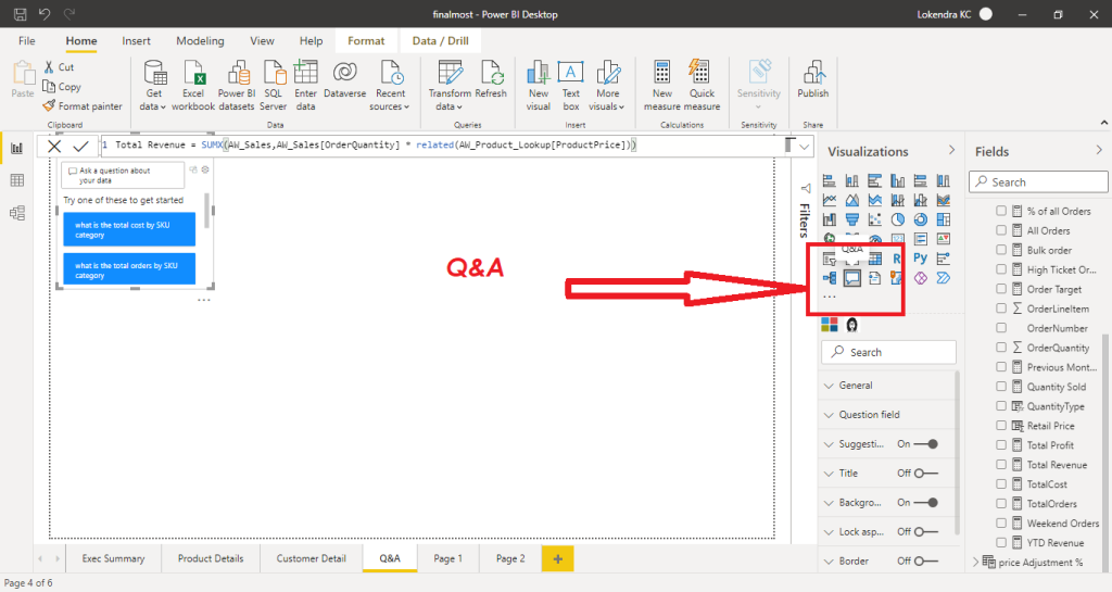
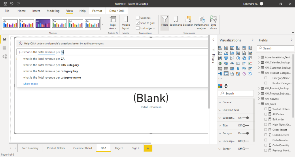
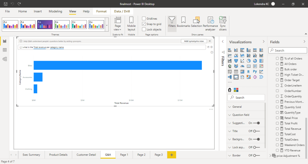
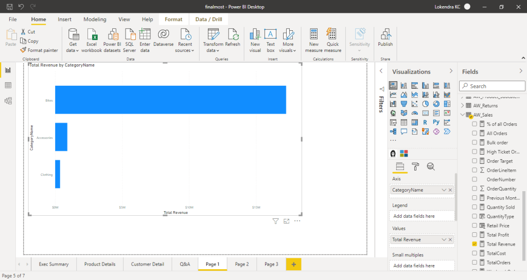
Additionally I used Power BI as well to create some meaningful visualizations.
Prepare Phase
Dataset is available under this license and can be found here .
I downloaded the data from the divvy trip data and stored in desktop.
- I renamed the folder to make it simple.
- I renamed all the files as per the standard naming conventions.
- I took 12 months of data and merged into the single folder.
Process and analyze Phase
In SSMS:
I used a variety of tools in-order to process and standardize the data. First I imported all the datasets in Microsoft sql server management studio. I appended all the datasets with the join query after making sure all the columns were matched and the datatypes were synchronized.
Problems : initially the datatypes were little bit different at the time of importing the data as the ssms automatically adjusted the datatype.
After join query I deleted the unwanted columns, for this particular case I deleted the latitude , longitude , start station Id , end Station Id.
I imported this data to the power BI to check the quality of columns as Power BI has capacity to autodetect errors, blank spaces. I replaced null station names to NA as to avoid confusion.
IN R :
I did the rest of the things in R
Here is the process and Steps
installing and reading Packages
library(tidyverse)
## — Attaching packages ————————————— tidyverse 1.3.1 —
## v ggplot2 3.3.5 v purrr 0.3.4
## v tibble 3.1.2 v dplyr 1.0.7
## v tidyr 1.1.3 v stringr 1.4.0
## v readr 1.4.0 v forcats 0.5.1
## — Conflicts —————————————— tidyverse_conflicts() —
## x dplyr::filter() masks stats::filter()
## x dplyr::lag() masks stats::lag()
library(lubridate)
##
## Attaching package: ‘lubridate’
## The following objects are masked from ‘package:base’:
##
## date, intersect, setdiff, union
library(ggplot2)
library(dplyr)
library(skimr)
Reading the cleaned data set /checking the Structure
`biketripdata` <- read.csv(“C:/Users/rayam/Desktop/Blogging/swapped capstone.csv”)
head(`biketripdata`)
## ride_id rideable_type started_at
## 1 169C7CEEFA777325 docked_bike 2021-04-17 04:19:01.0000000
## 2 169C90EB4F725D4F docked_bike 2021-07-16 14:04:39.0000000
## 3 169C9918EF1365A2 electric_bike 2021-06-11 14:50:27.0000000
## 4 169CA05C802CECBC electric_bike 2021-07-09 16:39:20.0000000
## 5 169CA7E2D1C4DF8A docked_bike 2020-08-01 11:38:55.0000000
## 6 169CAC157CA81FFE classic_bike 2021-06-04 17:06:05.0000000
## ended_at start_station_name
## 1 2021-04-17 04:24:02.0000000 Greenview Ave & Fullerton Ave
## 2 2021-07-16 14:59:07.0000000 Dusable Harbor
## 3 2021-06-11 15:02:48.0000000 Racine Ave & Washington Blvd
## 4 2021-07-09 17:04:37.0000000 East End Ave & 87th St
## 5 2020-08-01 11:39:14.0000000 Morgan Ave & 14th Pl
## 6 2021-06-04 17:27:25.0000000 Walsh Park
## end_station_name member_casual
## 1 Sheffield Ave & Wrightwood Ave casual
## 2 Lake Shore Dr & North Blvd casual
## 3 Wood St & Chicago Ave casual
## 4 Calumet Park member
## 5 Morgan Ave & 14th Pl casual
## 6 Humboldt Blvd & Armitage Ave casual
Checking the structure
str(biketripdata)
## ‘data.frame’: 4731081 obs. of 7 variables:
## $ ride_id : chr “169C7CEEFA777325” “169C90EB4F725D4F” “169C9918EF1365A2” “169CA05C802CECBC” …
## $ rideable_type : chr “docked_bike” “docked_bike” “electric_bike” “electric_bike” …
## $ started_at : chr “2021-04-17 04:19:01.0000000” “2021-07-16 14:04:39.0000000” “2021-06-11 14:50:27.0000000” “2021-07-09 16:39:20.0000000” …
## $ ended_at : chr “2021-04-17 04:24:02.0000000” “2021-07-16 14:59:07.0000000” “2021-06-11 15:02:48.0000000” “2021-07-09 17:04:37.0000000” …
## $ start_station_name: chr “Greenview Ave & Fullerton Ave” “Dusable Harbor” “Racine Ave & Washington Blvd” “East End Ave & 87th St” …
## $ end_station_name : chr “Sheffield Ave & Wrightwood Ave” “Lake Shore Dr & North Blvd” “Wood St & Chicago Ave” “Calumet Park” …
## $ member_casual : chr “casual” “casual” “casual” “member” …
Checking the data summary
skim(biketripdata)
Data summary
| Name | biketripdata |
| Number of rows | 4731081 |
| Number of columns | 7 |
| _______________________ | |
| Column type frequency: | |
| character | 7 |
| ________________________ | |
| Group variables | None |
Variable type: character
| skim_variable | n_missing | complete_rate | min | max | empty | n_unique | whitespace |
| ride_id | 0 | 1 | 16 | 16 | 0 | 4730872 | 0 |
| rideable_type | 0 | 1 | 11 | 13 | 0 | 3 | 0 |
| started_at | 0 | 1 | 27 | 27 | 0 | 4006808 | 0 |
| ended_at | 0 | 1 | 27 | 27 | 0 | 3989088 | 0 |
| start_station_name | 0 | 1 | 0 | 53 | 369182 | 739 | 0 |
| end_station_name | 0 | 1 | 0 | 53 | 407300 | 736 | 0 |
| member_casual | 0 | 1 | 6 | 6 | 0 | 2 | 0 |
Replace all the null value to N/A
biketripdata$start_station_name[biketripdata$start_station_name ==””]<- “N/A”
biketripdata$end_station_name[biketripdata$end_station_name ==””]<- “N/A”
As the date in not in data format I created new column as ridedate and assigned data type in ride_date
biketripdata$rideDate<-as.Date(biketripdata$started_at)
as we need the ride duration ; start date and end data are also assigned as Datetime data type
biketripdata$started_at<-as_datetime(biketripdata$started_at)
biketripdata$ended_at<-as_datetime(biketripdata$ended_at)
Creating the month , day , year , day of week as we need them further in analysis or the ride
biketripdata$month<-format(as.Date(biketripdata$rideDate),”%B”)
biketripdata$day <-format(as.Date(biketripdata$rideDate),”%d”)
biketripdata$year<-format(as.Date(biketripdata$rideDate),”%Y”)
biketripdata$day_of_week<-format(as.Date(biketripdata$rideDate),”%A”)
##checking the added column names again
colnames(biketripdata)
## [1] “ride_id” “rideable_type” “started_at”
## [4] “ended_at” “start_station_name” “end_station_name”
## [7] “member_casual” “rideDate” “month”
## [10] “day” “year” “day_of_week”
checking the quality of all things
skim(biketripdata)
Data summary
| Name | biketripdata |
| Number of rows | 4731081 |
| Number of columns | 12 |
| _______________________ | |
| Column type frequency: | |
| character | 9 |
| Date | 1 |
| POSIXct | 2 |
| ________________________ | |
| Group variables | None |
Variable type: character
| skim_variable | n_missing | complete_rate | min | max | empty | n_unique | whitespace |
| ride_id | 0 | 1 | 16 | 16 | 0 | 4730872 | 0 |
| rideable_type | 0 | 1 | 11 | 13 | 0 | 3 | 0 |
| start_station_name | 0 | 1 | 3 | 53 | 0 | 739 | 0 |
| end_station_name | 0 | 1 | 3 | 53 | 0 | 736 | 0 |
| member_casual | 0 | 1 | 6 | 6 | 0 | 2 | 0 |
| month | 0 | 1 | 3 | 9 | 0 | 12 | 0 |
| day | 0 | 1 | 2 | 2 | 0 | 31 | 0 |
| year | 0 | 1 | 4 | 4 | 0 | 2 | 0 |
| day_of_week | 0 | 1 | 6 | 9 | 0 | 7 | 0 |
Variable type: Date
| skim_variable | n_missing | complete_rate | min | max | median | n_unique |
| rideDate | 0 | 1 | 2020-08-01 | 2021-07-31 | 2021-04-05 | 365 |
Variable type: POSIXct
| skim_variable | n_missing | complete_rate | min | max | median | n_unique |
| started_at | 0 | 1 | 2020-08-01 00:00:01 | 2021-07-31 23:59:58 | 2021-04-05 13:41:29 | 4006808 |
| ended_at | 0 | 1 | 2020-08-01 00:04:41 | 2021-08-12 17:45:41 | 2021-04-05 14:03:51 | 3989088 |
##Creating the column – length of Ride and checking the summary
biketripdata$length_of_ride=difftime(biketripdata$ended_at,biketripdata$started_at)
summary(biketripdata$length_of_ride)
## Length Class Mode
## 4731081 difftime numeric
##Changing the column into numeric
biketripdata$length_of_ride=as.numeric(biketripdata$length_of_ride)
##filtering the length of ride less than 0 seconds
biketripdata_V2<-filter(biketripdata,length_of_ride>0)
##minimum Length of ride and maximum length of ride
min(biketripdata_V2$length_of_ride)
## [1] 1
max(biketripdata_V2$length_of_ride)
## [1] 3356649
##average length of ride along with min and max
biketripdata_V2%>%summarise(min_ride_length=min(length_of_ride),max_ride_length=max(length_of_ride),average_length_ride=mean(length_of_ride))
## min_ride_length max_ride_length average_length_ride
## 1 1 3356649 1606.376
##length of Ride by member_type
aggregate(biketripdata_V2$length_of_ride~biketripdata_V2$member_casual,FUN = mean)
## biketripdata_V2$member_casual biketripdata_V2$length_of_ride
## 1 casual 2267.697
## 2 member 1077.608
aggregate(biketripdata_V2$length_of_ride~biketripdata_V2$member_casual,FUN = median)
## biketripdata_V2$member_casual biketripdata_V2$length_of_ride
## 1 casual 1079
## 2 member 629
aggregate(biketripdata_V2$length_of_ride~biketripdata_V2$member_casual,FUN = max)
## biketripdata_V2$member_casual biketripdata_V2$length_of_ride
## 1 casual 3356649
## 2 member 2005282
Before proceeding with the weekday analysis , lets sort out the things by weekday
biketripdata_V2$day_of_week<-ordered(biketripdata_V2$day_of_week,levels=c(‘Monday’,’Tuesday’,’Wednesday’,’Thursday’,’Friday’,’Saturday’,’Sunday’))
##mean length of ride by membertype and day of week
aggregate(biketripdata_V2$length_of_ride~biketripdata_V2$member_casual+biketripdata_V2$day_of_week,FUN=mean)
## biketripdata_V2$member_casual biketripdata_V2$day_of_week
## 1 casual Monday
## 2 member Monday
## 3 casual Tuesday
## 4 member Tuesday
## 5 casual Wednesday
## 6 member Wednesday
## 7 casual Thursday
## 8 member Thursday
## 9 casual Friday
## 10 member Friday
## 11 casual Saturday
## 12 member Saturday
## 13 casual Sunday
## 14 member Sunday
## biketripdata_V2$length_of_ride
## 1 2170.0176
## 2 855.2013
## 3 1958.3320
## 4 832.1721
## 5 2527.8431
## 6 2112.8943
## 7 1933.2624
## 8 831.0379
## 9 2088.6483
## 10 866.7661
## 11 2374.0114
## 12 971.0323
## 13 2550.7374
## 14 1003.5724
##Maximum length of ride by member type and weekday name
aggregate(biketripdata_V2$length_of_ride~biketripdata_V2$member_casual+biketripdata_V2$day_of_week,FUN=max)
## biketripdata_V2$member_casual biketripdata_V2$day_of_week
## 1 casual Monday
## 2 member Monday
## 3 casual Tuesday
## 4 member Tuesday
## 5 casual Wednesday
## 6 member Wednesday
## 7 casual Thursday
## 8 member Thursday
## 9 casual Friday
## 10 member Friday
## 11 casual Saturday
## 12 member Saturday
## 13 casual Sunday
## 14 member Sunday
## biketripdata_V2$length_of_ride
## 1 2033524
## 2 2005282
## 3 2335375
## 4 433425
## 5 3257001
## 6 1742998
## 7 2946429
## 8 1682901
## 9 3341501
## 10 713853
## 11 3356649
## 12 990269
## 13 3235296
## 14 1870176
sorting the data by months
biketripdata_V2$month<-ordered(biketripdata_V2$month,levels=c(‘January’, ‘February’, ‘March’, ‘April’, ‘May’, ‘June’, ‘July’, ‘August’, ‘September’, ‘October’, ‘November’, ‘December’))
mean ride length by months and Rider type
aggregate(biketripdata_V2$length_of_ride~biketripdata_V2$member_casual+biketripdata_V2$month,FUN=mean)
## biketripdata_V2$member_casual biketripdata_V2$month
## 1 casual January
## 2 member January
## 3 casual February
## 4 member February
## 5 casual March
## 6 member March
## 7 casual April
## 8 member April
## 9 casual May
## 10 member May
## 11 casual June
## 12 member June
## 13 casual July
## 14 member July
## 15 casual August
## 16 member August
## 17 casual September
## 18 member September
## 19 casual October
## 20 member October
## 21 casual November
## 22 member November
## 23 casual December
## 24 member December
## biketripdata_V2$length_of_ride
## 1 1541.0754
## 2 772.3612
## 3 2962.6862
## 4 1081.4072
## 5 2289.6329
## 6 838.2321
## 7 2281.5631
## 8 881.4281
## 9 2294.1080
## 10 878.4114
## 11 2227.5393
## 12 880.7155
## 13 1967.5752
## 14 854.4311
## 15 2686.9206
## 16 1004.9515
## 17 2287.2709
## 18 927.9440
## 19 1809.8691
## 20 839.4808
## 21 3439.3526
## 22 3795.2678
## 23 1610.9252
## 24 764.6206
##counting the total ride per month for the member types
biketripdata_V2%>%count(month,member_casual)
## month member_casual n
## 1 January casual 18117
## 2 January member 78713
## 3 February casual 10130
## 4 February member 39488
## 5 March casual 84029
## 6 March member 144457
## 7 April casual 136590
## 8 April member 200607
## 9 May casual 256888
## 10 May member 274693
## 11 June casual 370639
## 12 June member 358895
## 13 July casual 442019
## 14 July member 380322
## 15 August casual 289608
## 16 August member 332642
## 17 September casual 230669
## 18 September member 302230
## 19 October casual 144994
## 20 October member 243619
## 21 November casual 88169
## 22 November member 171897
## 23 December casual 29998
## 24 December member 101189
counting the ridable type for Riders
biketripdata_V2 %>%count(member_casual,rideable_type)
## member_casual rideable_type n
## 1 casual classic_bike 695208
## 2 casual docked_bike 760291
## 3 casual electric_bike 646351
## 4 member classic_bike 1090190
## 5 member docked_bike 797881
## 6 member electric_bike 740681
Visualization Phase
Summary of the average ride length per day of week and Rider type
biketripdata_V2%>%group_by(member_casual,day_of_week)%>%summarise(average_ride_length=mean(length_of_ride))%>%
ggplot(aes(x=member_casual,y=average_ride_length,fill=day_of_week)) +
geom_bar(position=”Dodge”,stat = “identity”) +
labs(title=”distribution of average ride length by week”,subtitle=”sorted by membership”)
## `summarise()` has grouped output by ‘member_casual’. You can override using the `.groups` argument.

Total Ride duration per day of week and rider type
biketripdata_V2%>%group_by(member_casual,day_of_week)%>%summarise(total_ride_duration=mean(length_of_ride))%>%
ggplot(aes(x=member_casual,y=total_ride_duration,fill=day_of_week)) +
geom_bar(position=”Dodge”,stat = “identity”) +
labs(title=”average ride length by day of week”,subtitle=”sorted by membership”)

Trips less than 5 minutes ie. 5*60 =300 secs
biketripdata_V2%>%group_by(day_of_week,member_casual)%>%filter(length_of_ride<300 )%>%
summarise(average_ride_length=mean(length_of_ride))%>%
ggplot(aes(x=day_of_week,y=average_ride_length, fill=member_casual)) +
geom_bar(position=’Dodge’,stat=’identity’) +
labs(title=”Average ride length among different members by day of week which is less than 5 mins “,subtitle=”Membership comparision”)

Trips more than 5 mins
biketripdata_V2%>%group_by(day_of_week,member_casual)%>%filter(length_of_ride>300 )%>%
summarise(average_ride_length=mean(length_of_ride))%>%
ggplot(aes(x=day_of_week,y=average_ride_length, fill=member_casual)) +
geom_bar(position=’Dodge’,stat=’identity’) +
labs(title=”Average ride length among different members by day of week which is less than 5 mins “,subtitle=”Membership comparision”)

Total Rides per month number and rider type
biketripdata_V2%>%group_by(month,member_casual)%>%summarise(Ridenumbers=n())%>%
ggplot(aes(x=month,y=Ridenumbers, fill=member_casual)) +
geom_bar(position=’Dodge’,stat=’identity’) +
labs(title=”distribution of ride numbers by month”,subtitle=”Membership comparision”)

Total length of Ride per month among rider types
biketripdata_V2%>%group_by(month,member_casual)%>%summarise(totalrideduration=sum(length_of_ride))%>%
ggplot(aes(x=month,y=totalrideduration, fill=member_casual)) +
geom_bar(position=’Dodge’,stat=’identity’) +
labs(title=”distribution of total ride duration by month”,subtitle=”Membership comparision”)

Total Rides per year and membership type
biketripdata_V2%>%group_by(year,member_casual)%>%summarise(Ridenumbers=n())%>%
ggplot(aes(x=year,y=Ridenumbers, fill=member_casual)) +
geom_bar(position=’Dodge’,stat=’identity’) +
labs(title=”distribution of ride numbers by year”,subtitle=”Membership comparision”)

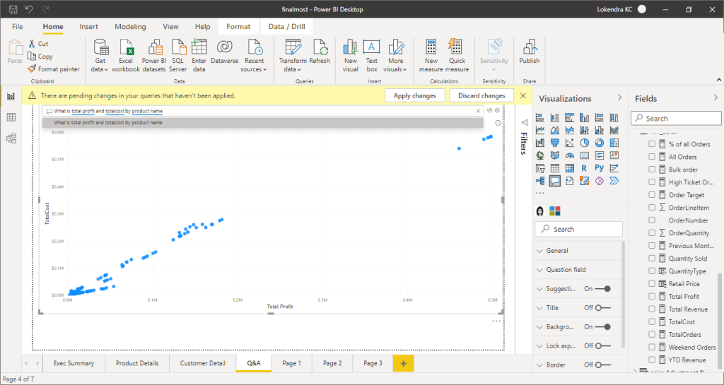
Alternatively I created the visualization in Power BI as well to utilize my skills ,


ACT Phase
Now on the basis of our above steps ask , prepare , process, analyze , share I have come into following recommendations :
- Tuesdays and Sundays are more effective in case of casual riders whereas for riders with membership , Tuesday is the peak. So , Tuesday is the most effective day for marketing and we can bring some discount or promotion package.
- Riders with membership prefer the short rides and we can see there are more riders with membership more than casual riders whereas casual riders prefer lengthy rides. So we can encourage discounts on short rides as well.
- Between June and July there is a peak in numbers of rides so promotion and packages for membership is recommended at that time.
- Base – 2132 W Hubbard Warehouse,Hubbard St Bike checking , Indiana Ave , Lake shore Dr , Michigan ave, millennium park are the most visited locations and marketing can be strictly focused on that area.
5. The most popular bikes are Docked bike which are preferred means of bike for casual riders so company can focus more on Docked bikes.